How to Protect Cells in Excel [ Updated 2019 ]

Think of your boss needing you to ensure a whole workbook, yet in addition, needs to have the option to change a couple of cells after you have got the protection enabled on the workbook.

Lock cells to protect them – Lock or unlock specific areas of a protected worksheet

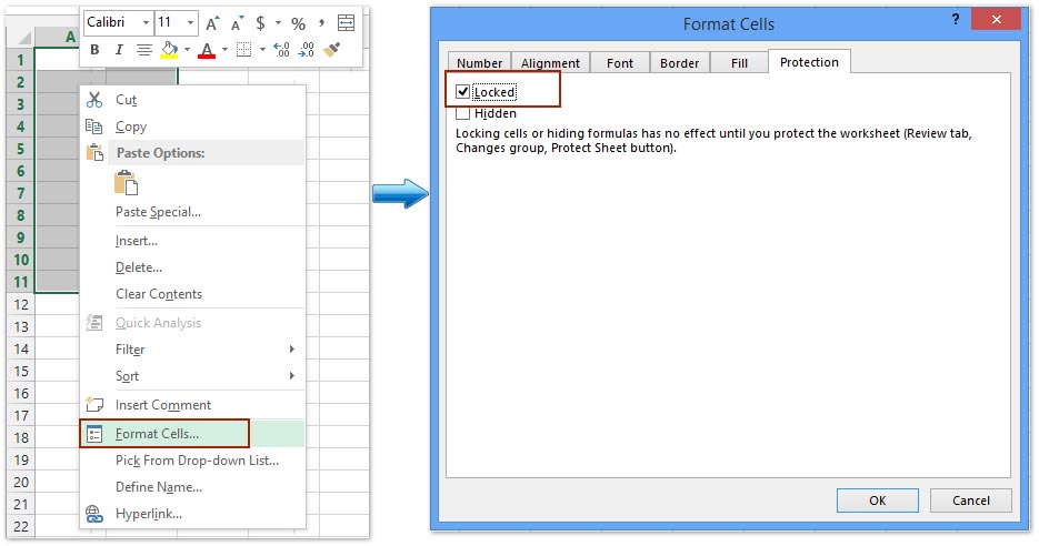
Before you get done with enabling the password protection or security, you had opened a few cells in the workbook. Since your boss is finished with the workbook, you are able to lock the cells. Please make sure to go through these steps mentioned below in order to lock cells in the worksheet:

1. At first, choose the cells, which you need to lock.
2. In the Alignment group, on the Home tab, go ahead click the small arrow in order to run the Format Cells popup window.
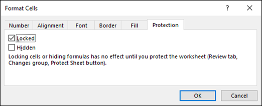
3. Ensure to choose the Locked checkbox, on the Protection tab, and then move ahead and click OK in order to close this popup.

Important Note: In the case, if you attempt these given steps on a worksheet or workbook, which you haven’t still kept protected, you will be able to witness the cells that have been locked already. This points to you that the cells are more than just ready for locking them when you are trying to protect the worksheet or workbook.

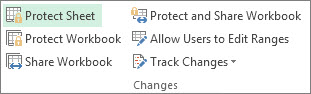
1. In the Changes group, in the Review tab in the ribbon, choose either Protect Sheet or just go for Protect Workbook, and now, you can reapply for protection. So go ahead and see Protect a workbook or protect a worksheet.

Tip: It’s one of the best practices in order to unlock the cells, which you would like to change before you opt for the protection of a workbook or a worksheet, but you are also able to unlock them once you are done applying for protection. In order to remove protection, just go ahead and remove the password.

Apart from the protection of the workbooks and/or worksheets, you will also be able to protect formulas. Also, Excel for the web is not able to lock cells or any particular areas of a workbook or worksheet.

In the case, if you need locking the cells or to protect any particular areas, just click Open in Excel and then just lock cells in order to protect them or simply lock or unlock particular areas of a worksheet that is protected.

Lock or unlock specific areas of a protected worksheet

Protecting a worksheet will tend to lock all cells by default and hence, none of these cells will remain editable. In order to enable a bit c of ell editing especially when keeping other cells locked, to unlock all of these cells is possible. You are able to lock any particular cells as well as ranges before protecting a worksheet and you can also enable certain users in order to edit, optionally, in just specifies ranges from the sheet which has been protected. If you have encrypted excel spreadsheet then do not forget the password or else you may lose data from the spreadsheet. There are several tricks to recover your excel password to get your spreadsheet in action.

Only Lock Specific Cells or Ranges in the Protected Worksheet

Follow the below-mentioned steps:

If the worksheet has been protected, you may opt for the following steps:

1. At first, click Unprotect Sheet on the Review tab (in the Changes group).

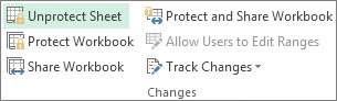
Tap the Protect Sheet button in order to Unprotect Sheet when the worksheet gets protected.

2. Enter the password in order to unprotect a worksheet, if prompted.

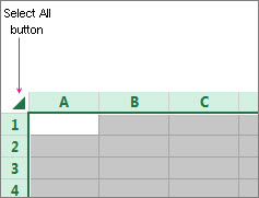
3. Make a selection of the whole worksheet just by clicking the button “Select all”.

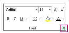
4. Click the Format Cell Font popup launcher, on the Home tab. You may also tap Ctrl+Shift+F or Ctrl+1.

5. In the Protection tab, in the Format Cells popup, ensure to uncheck the Locked box, go ahead and then click OK. This will help in unlocking all the cells on a worksheet once you have protected a worksheet. Now, you will be able to choose the cells that you particularly need to lock.

1. Choose the cells only which you have to lock on the worksheet.
2. Run the Format Cells popup window once again (Ctrl+Shift+F).
3. At this point of time, on the Protection tab, ensure to check the Locked box, go ahead and then click OK.
4. Click Protect Sheet on the Review tab.

1. Select the elements which you need users to make about a change in the Allow all users of the worksheet to list.

More information related to worksheet elements:

Clear this checkbox To prevent users from Select locked cells Taking the pointer to the cells for which the Locked check box has been chosen of the Format Cells dialog box on the Protection tab. Users are permitted to choose locked cells by default. Select unlocked cells Taking the pointer to the cells for which the Locked check box has been cleared of the Format Cells dialog box on the Protection tab. Users are permitted to choose locked cells by default and they are able to press the TAB key for moving, on a protected worksheet, between the unlocked cells. Format cells Modifying any of the options in the Conditional Formatting dialog boxes or Format Cells. If you have applied for the conditional formats before protecting the worksheet, the formatting will continue changing when any user will enter a value which will be satisfying a different condition. Format columns With the use of any column formatting commands that includes hiding columns or changing column width (Home tab, Format button, Cells group). Format rows With the use of any row formatting commands that includes changing row height or hiding rows (Home tab, Format button, Cells group). Insert columns Inserting columns. Insert rows Inserting rows. Insert hyperlinks Inserting newer hyperlinks, including the unlocked cells. Delete columns Deleting columns. If Delete columns have been protected and Insert columns have not been protected, any user is able to insert columns, which he or she can’t delete. Delete rows Deleting rows. If Delete rows have been protected and Insert rows have not been protected, any user is able to insert rows, which he or she can’t delete. Sort Using any commands in order to sort data (Data tab, Sort & Filter group). Users can’t sort ranges (regardless of this setting), which consists of locked cells on a protected worksheet. Use AutoFilter With the use of the drop-down arrows for changing the filter on ranges when AutoFilters get applied. Users aren’t able to apply or remove AutoFilters (regardless of this setting) on a protected worksheet. Use PivotTable reports Formatting, refreshing, changing the layout, or otherwise modifying PivotTable reports, or to create new reports. Edit objects Doing any of the below: Making modifications to graphic objects, which include maps, shapes, text boxes, embedded charts, and controls that you have not unlocked before protecting the worksheet. For example, if a worksheet comes with a button which runs a macro, you are able to click the button in order to run the macro, but you aren’t able to delete the button. Making any modifications like formatting, to the embedded chart. The chart keeps on getting updated when a user changes its source data. Editing or adding comments. Edit scenarios Considering various scenarios that have been hidden, making modifications to scenarios which you have prevented modifications to, and then deletion of these scenarios. Users are allowed to modify the values in the ever-changing cells, in the case, if the cells haven’t been protected, move ahead and add new scenarios.

Chart sheet elements

Select this checkbox	To prevent users from
Contents	Making modifications to items which have been a part of the chart, for example, axes, data series, and legends. The chart keeps on reflecting modifications which are made to its source data.
Objects	Making modifications to graphic objects that include text boxes, shapes, and controls — till the time you get the objects unlocked before protecting the chart sheet.

1. Type a password in the Password to unprotect sheet box, for the sheet, and then click OK, and now retype the password in order to confirm it.
   • The password is optional though. If you are not supplying a password, a user is able to unprotect the sheet easily and modify the protected elements.
   • Ensure choosing a password that you will be able to remember easily and won’t forget easily because, in the case, if you lose your password, you will not have the access to your protected elements that are there on the worksheet.

Unlock Ranges on the Protected Worksheet for Users for Editing

In order to give certain users allowance for editing ranges in a worksheet which is protected, your PC must be running Microsoft Windows XP or older version, and your PC must also be in a domain. So in the place of using allowances that ask for a domain, you will be able to specify a password also for the range.

1. Make a selection of the worksheet that you need to protect.
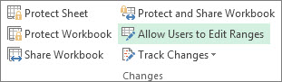
2. In the Changes group on the Review tab, move further and press Allow Users to Edit Ranges. This command is just available when a worksheet hasn’t been protected.

1. Perform one of the below:
   • In order to add a latest editable range, tap New.
   • In order to modify an already existing editable range, make a selection of it in the Ranges unlocked by a password when a sheet is protected box, go ahead and then click Modify.
   • In order to delete an editable range, make a selection of it in the Ranges unlocked by a password when the sheet is protected box, go ahead and then press Delete.
2. Type the name in the Title box for the range which you have got to unlock.
3. In the box that says Refers to cells, type (=), an equal sign, and now type the range reference that you have got to unlock. Moreover, you are also able to click the Collapse Dialog button, make a selection of the range in a worksheet, and now click the Collapse Dialog button once again for returning to the dialog box.
4. For the access to the password, type a password in the Range password box, which will allow you access to the range. Specifying a password is not a compulsion but it’s optional when you are planning to utilize access permissions. With the use of a password that allows you seeing user credentials of the authorized person who is able to edit the range.
5. In order to access permissions, just click Permissions, and now click Add.
6. In the Enter, the object names to select (examples) box, go ahead and type user names who you have got to allow editing the ranges. In order to see how the names of the users would be entered, simply press examples. Also, for the verification of if the names are correct or not, go ahead and click Check Names.
7. Press OK.
8. For specifying the type of allowance for the user who has been selected by you, clear or select the Deny or Allow checkboxes, in the Permissions box, and then press Apply.
9. Now, press OK twice. In the case, if you are prompted for any password, go ahead and type the password which you have specified.
10. Now, click Protect Sheet in the Allow Users to Edit Ranges dialog box.
11. Choose the elements which you wish the users to be able to modify in the Allow all users of this worksheet to list.

More information related to worksheet elements:

Clear this checkbox To prevent users from Select locked cells Taking the pointer to the cells for which the Locked checkbox has been chosen of the Format Cells dialog box on the Protection tab. Users are permitted to choose locked cells by default. Select unlocked cells Taking the pointer to the cells for which the Locked checkbox has been cleared of the Format Cells dialog box on the Protection tab. Users are permitted to choose locked cells by default and they are able to press the TAB key for moving, on a protected worksheet, between the unlocked cells. Format cells Modifying any of the options in the Conditional Formatting dialog boxes or Format Cells. If you have applied for the conditional formats before protecting the worksheet, the formatting will continue changing when any user will enter a value which will be satisfying a different condition. Format columns With the use of any column formatting commands that includes hiding columns or changing column width (Home tab, Format button, Cells group). Format rows With the use of any row formatting commands that includes changing row height or hiding rows (Home tab, Format button, Cells group). Insert columns Inserting columns. Insert rows Inserting rows. Insert hyperlinks Inserting newer hyperlinks, including the unlocked cells. Delete columns Deleting columns. If Delete columns have been protected and Insert columns have not been protected, any user is able to insert columns, which he or she can’t delete. Delete rows Deleting rows. If Delete rows have been protected and Insert rows have not been protected, any user is able to insert rows, which he or she can’t delete. Sort Using any commands in order to sort data (Data tab, Sort & Filter group). Users can’t sort ranges (regardless of this setting), which consists of locked cells on a protected worksheet. Use AutoFilter With the use of the drop-down arrows for changing the filter on ranges when AutoFilters get applied. Users aren’t able to apply or remove AutoFilters (regardless of this setting) on a protected worksheet. Use PivotTable reports Formatting, refreshing, changing the layout, or otherwise modifying PivotTable reports, or to create new reports. Edit objects Doing any of the below: Making modifications to graphic objects, which include maps, shapes, text boxes, embedded charts, and controls that you have not unlocked before protecting the worksheet. For example, if a worksheet comes with a button which runs a macro, you are able to click the button in order to run the macro, but you aren’t able to delete the button. Making any modifications like formatting, to the embedded chart. The chart keeps on getting updated when a user changes its source data. Editing or adding comments. Edit scenarios Considering various scenarios that have been hidden, making modifications to scenarios which you have prevented modifications to, and then deletion of these scenarios. Users are allowed to modify the values in the ever-changing cells, in the case, if the cells haven’t been protected, move ahead and add new scenarios.

Chart sheet elements

Select this checkbox	To prevent users from
Contents	Making modifications to items which have been a part of the chart, for example, axes, data series, and legends. The chart keeps on reflecting modifications which are made to its source data.
Objects	Making modifications to graphic objects that include text boxes, shapes, and controls — till the time you get the objects unlocked before protecting the chart sheet.

1. Type a password in the Password to unprotect sheet box, for the sheet, and then click OK, and now retype the password in order to confirm it.

• The password is optional though. If you are not supplying a password, a user is able to unprotect the sheet easily and modify the protected elements.
• Ensure choosing a password that you will be able to remember easily and won’t forget easily because, in the case, if you lose your password, you will not have the access to your protected elements that are there on the worksheet.
• In the case, if you find that a cell belongs to more than a single range; users who have been authorized for editing one of those ranges are allowed to edit the cell.
• If a user attempts to edit multiple cells at one time and has got authorized for editing a few but not all of the cells then the user will be prompted for editing the cells one at a time.

You should also know about how to merge cells in excel as we have a specific article about that.